From MLE to Variational Inference

Table of contents

Introduction: The Foundation of Generative Modeling

Understanding modern generative models requires grasping a fundamental progression in machine learning theory: from simple maximum likelihood estimation to sophisticated variational inference methods. This mathematical journey reveals how we moved from modeling observable data directly to learning complex latent representations that capture the hidden structure of our world.

The path we’ll explore connects three crucial concepts: Maximum Likelihood Estimation as our optimization foundation, Latent Variable Models as our structural framework, and Variational Inference as our computational solution. Each builds upon the previous, creating a coherent theoretical narrative that explains why modern generative models like Variational Autoencoders work the way they do.

Part I: Maximum Likelihood Learning - The Foundation

The Core Principle

Maximum Likelihood Estimation (MLE) forms the bedrock of modern generative modeling. Given a dataset $\mathcal{D} = \{x^{(1)}, x^{(2)}, ..., x^{(n)}\}$, our goal is to find model parameters $\theta$ that maximize the likelihood of observing our data:

In practice, we maximize the log-likelihood for computational convenience:

The Connection to KL Divergence

A profound insight emerges when we recognize that MLE is equivalent to minimizing the KL divergence between the true data distribution $p_{data}(x)$ and our model distribution $p_\theta(x)$:

This connection reveals why MLE is so fundamental: we’re not just fitting parameters, we’re finding the model distribution that best approximates reality.

For a detailed derivation of this connection and its implications (including the crucial asymmetry of KL divergence), see my previous post on Maximum Likelihood Learning and the KL Connection.

From Expected to Empirical Log-Likelihood

In practice, we don’t know the true data distribution $p_{data}(x)$. Instead, we approximate the expected log-likelihood with the empirical log-likelihood using our dataset:

Maximum likelihood learning then becomes:

The Bias-Variance Tradeoff

A crucial challenge in MLE is balancing model complexity. Consider the bias-variance decomposition:

• Bias: Error from model assumptions (underfitting)
• Variance: Error from sensitivity to training data (overfitting)
• Noise: Irreducible error

Simple models (high bias, low variance) underfit, while complex models (low bias, high variance) overfit. The art lies in finding the sweet spot.

Optimization Through Gradient Descent

MLE objectives are typically optimized using gradient descent:

where $\eta$ is the learning rate. The gradient points in the direction of steepest increase in likelihood, guiding us toward better parameter values.

For neural networks, we use backpropagation to compute gradients efficiently, enabling the deep learning revolution in generative modeling.

Part II: Latent Variable Models - Capturing Hidden Structure

Beyond Observable Variables

While MLE works well for simple distributions, real-world data often has underlying structure that isn’t directly observable. Consider images: the pixels we see are generated by hidden factors like object identity, lighting, pose, and style. Latent Variable Models capture this intuition by introducing unobserved variables $z$ that explain the data generation process.

The fundamental latent variable model assumes:

where:

• $p(z)$ is the prior over latent variables
• $p_\theta(x|z)$ is the likelihood of data given latents
• $p_\theta(x)$ is the marginal likelihood we observe

The Intractability Problem

This integral is the heart of the challenge. For complex models like neural networks, this integral becomes intractable:

We cannot directly optimize $\log p_\theta(x)$ because we cannot compute it.

Example: Mixture of Gaussians

Consider a simple latent variable model - Mixture of Gaussians:

Even this simple case requires summing over all mixture components. For neural networks with continuous latent spaces, the intractability becomes severe.

The Posterior Inference Challenge

Even if we could compute $p_\theta(x)$, we face another challenge: computing the posterior $p_\theta(z|x)$ for inference:

This posterior tells us what latent factors likely generated a given observation - crucial for understanding and manipulating our model.

Part III: Variational Inference - The Computational Solution

Approximating the Intractable

Variational inference provides an elegant solution to intractability. Instead of computing the exact posterior $p_\theta(z|x)$, we approximate it with a simpler distribution $q_\phi(z|x)$ parameterized by $\phi$.

The key insight is to optimize this approximation to be as close as possible to the true posterior:

Deriving the Evidence Lower Bound (ELBO)

The breakthrough comes from a clever mathematical manipulation. Starting with the log-likelihood:

We multiply and divide by our approximation $q_\phi(z|x)$:

Applying Jensen’s inequality (since log is concave):

Understanding Jensen’s Inequality: The key mathematical insight here is that the logarithm function is concave, meaning that for any convex combination of points, the function value at that combination is greater than or equal to the convex combination of function values. This fundamental property enables the ELBO derivation.

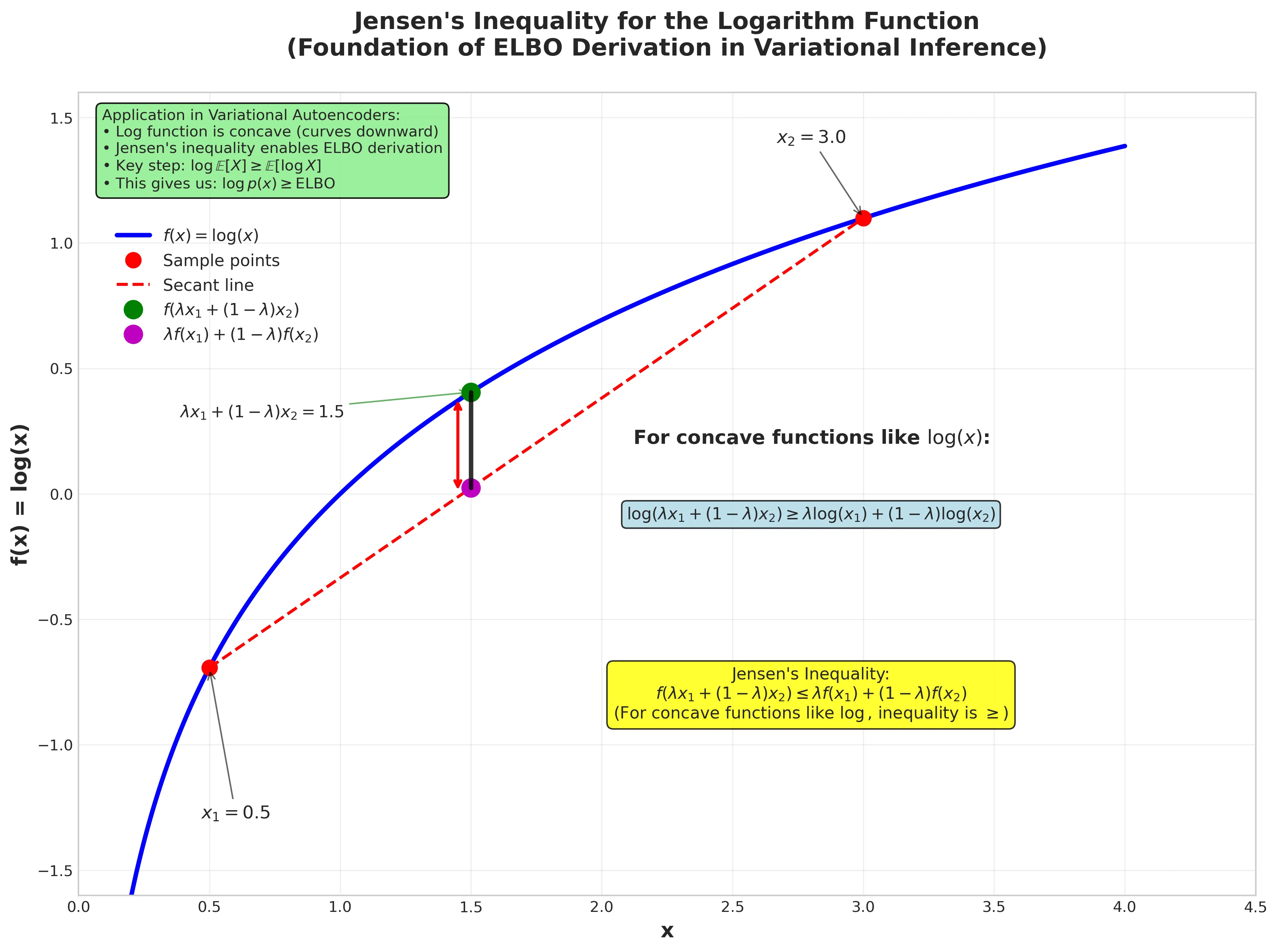
Figure: Jensen’s inequality demonstration for the logarithm function. The plot shows how the expectation of the log (green point) lies above the log of the expectation (magenta point) for concave functions. This mathematical property is crucial for deriving the ELBO. View source code

This gives us the Evidence Lower Bound (ELBO):

Rearranging terms: We can rewrite this by using the factorization $p_\theta(x,z) = p_\theta(x|z)p(z)$:

This final form reveals the ELBO’s intuitive structure as a balance between reconstruction and regularization.

Understanding the ELBO

The ELBO decomposes into two intuitive terms:

1. Reconstruction Term: $\mathbb{E}_{q_\phi(z|x)}[\log p_\theta(x|z)]$

   • Measures how well we can reconstruct $x$ from latent $z$
   • Encourages the decoder to be accurate

2. Regularization Term: $D_{KL}(q_\phi(z|x) || p(z))$

   • Keeps the approximate posterior close to the prior
   • Prevents overfitting and ensures smooth latent space

The Variational Gap

The difference between the true log-likelihood and the ELBO is exactly the KL divergence we wanted to minimize. To see where this comes from, let’s start with the definition of KL divergence between our approximate posterior and the true posterior:

Using Bayes’ rule, we know that $p_\theta(z|x) = \frac{p_\theta(x,z)}{p_\theta(x)}$, so:

Therefore:

Why maximizing the ELBO simultaneously improves both model and approximation:

Since $D_{KL}(q_\phi(z|x) || p_\theta(z|x)) \geq 0$ always, we have:

When we maximize $\mathcal{L}(\theta,\phi)$, we can do so by:

1. Improving our model (w.r.t. $\theta$): Increasing $\mathcal{L}(\theta,\phi)$ forces $\log p_\theta(x)$ to increase (since the KL term is non-negative), meaning our model assigns higher probability to the observed data.

2. Improving our approximation (w.r.t. $\phi$): Increasing $\mathcal{L}(\theta,\phi)$ while keeping $\log p_\theta(x)$ fixed forces the KL divergence $D_{KL}(q_\phi(z|x) || p_\theta(z|x))$ to decrease, meaning our approximate posterior $q_\phi(z|x)$ becomes closer to the true posterior $p_\theta(z|x)$.

This is the beauty of variational inference: a single objective simultaneously pushes us toward both a better model and a better approximation!

Part IV: Variational Autoencoders - The Practical Realization

From Theory to Architecture

Variational Autoencoders (VAEs) represent the practical implementation of the variational inference framework we’ve developed. In the landscape of generative models, VAEs stand out for their elegant probabilistic approach to learning latent representations of data. Unlike autoregressive models that predict data sequentially, VAEs learn a continuous latent space, which allows for powerful generation and manipulation of data.

The VAE Architecture

A VAE consists of two neural networks working in tandem:

Encoder $q_\phi(z|x)$:

• Takes input data $x$ and outputs parameters of a distribution over latent codes
• Typically outputs mean $\mu_\phi(x)$ and log-variance $\log\sigma_\phi^2(x)$
• Architecture: CNN for images, transformer layers for text, MLP for tabular data

Decoder $p_\theta(x|z)$:

• Takes latent code $z$ and generates reconstruction of original data
• For images: often outputs pixel intensities or logits
• Architecture: Transpose CNN for images, autoregressive decoder for sequences

The VAE Objective in Practice

The ELBO we derived translates directly into the VAE training objective:

This decomposes into:

1. Reconstruction Loss: How well can we reconstruct the input from its latent representation?
2. KL Regularization: How close is our learned posterior to the simple prior?

The beauty of this objective is that it naturally balances two competing goals:

• Reconstruction fidelity: The decoder should accurately reproduce the input
• Latent space structure: The encoder should produce well-organized latent codes

Understanding the Latent Space

The KL regularization term serves a crucial purpose beyond mathematical convenience. By forcing $q_\phi(z|x) \approx p(z) = \mathcal{N}(0,I)$, we ensure:

• Smooth interpolation: Moving between points in latent space produces meaningful transitions
• Generative capability: We can sample new data by drawing $z \sim p(z)$ and decoding
• Regularized learning: The model can’t “cheat” by memorizing unique codes for each input

When the bound becomes tight (i.e., when $q_\phi(z|x) \approx p_\theta(z|x)$), the VAE achieves optimal performance:

The gap between ELBO and true log-likelihood is exactly this approximation quality.

Part V: Advanced Variational Techniques

Importance Weighted Autoencoders (IWAE)

The ELBO can sometimes be a loose bound. IWAE provides a tighter bound using multiple samples:

Key properties:

• For $K=1$: reduces to standard ELBO
• For $K>1$: provides strictly tighter bound
• As $K \to \infty$: approaches true log-likelihood

The bound hierarchy is:

β-VAE: Controlling Disentanglement

The β-VAE modifies the ELBO to control the latent space structure:

Different β values yield different behaviors:

• β = 1: Standard VAE (balanced reconstruction and regularization)
• β > 1: Emphasizes disentanglement (individual latent dimensions capture distinct factors)
• β < 1: Emphasizes reconstruction quality

This provides a principled way to trade off between reconstruction fidelity and interpretable representations.

Semi-Supervised VAE (SSVAE)

SSVAE extends VAEs to leverage both labeled and unlabeled data:

For labeled data:

For unlabeled data:

where $\mathcal{H}[q(y|x)]$ is the entropy encouraging diverse predictions.

Fully Supervised VAE (FSVAE)

When full supervision is available, we can condition the entire model on labels:

This allows the model to learn label-specific latent structures.

Part VI: The Reparameterization Trick - Making It Trainable

The Gradient Problem

A crucial challenge in training variational models is that the ELBO involves expectations over the approximate posterior $q_\phi(z|x)$. We need gradients with respect to $\phi$, but sampling operations aren’t differentiable.

The Solution

The reparameterization trick transforms the sampling process. Instead of sampling directly from $q_\phi(z|x)$, we:

1. Sample noise from a fixed distribution: $\epsilon \sim p(\epsilon)$
2. Apply a deterministic transformation: $z = g_\phi(\epsilon, x)$

For Gaussian $q_\phi(z|x) = \mathcal{N}(\mu_\phi(x), \sigma_\phi^2(x))$:

Now gradients can flow through the deterministic path from $\phi$ to the loss.

Monte Carlo Estimation

With reparameterization, we estimate the ELBO using Monte Carlo:

where $z^{(l)} = \mu_\phi(x) + \sigma_\phi(x) \odot \epsilon^{(l)}$.

Part VII: Practical Implementation Insights

Neural Network Architectures

Encoder $q_\phi(z|x)$:

• Input: data $x$
• Outputs: mean $\mu_\phi(x)$ and log-variance $\log\sigma_\phi^2(x)$
• Architecture: CNN for images, MLP for tabular data

Decoder $p_\theta(x|z)$:

• Input: latent code $z$
• Output: reconstruction parameters
• For images: often outputs logits for each pixel

Key Implementation Functions

Key implementation functions include:

def sample_gaussian(mu, log_var):
    """Sample from Gaussian using reparameterization trick"""
    std = torch.exp(0.5 * log_var)
    eps = torch.randn_like(std)
    return mu + eps * std

def log_normal(x, mu, log_var):
    """Compute log probability of Gaussian"""
    return -0.5 * (log_var + (x - mu).pow(2) / log_var.exp())

def negative_elbo_bound(x_hat, x, mu, log_var):
    """Compute negative ELBO for optimization"""
    reconstruction_loss = F.binary_cross_entropy(x_hat, x, reduction='sum')
    kl_divergence = -0.5 * torch.sum(1 + log_var - mu.pow(2) - log_var.exp())
    return reconstruction_loss + kl_divergence

Training Considerations

Optimization: Adam optimizer typically works well with learning rates around 1e-3 to 1e-4.

KL Annealing: Gradually increase the KL weight from 0 to 1 during training to avoid posterior collapse:

where $\beta(t)$ increases from 0 to 1 over training.

Part VIII: Connecting Theory to Practice

From MLE to VAE

The progression we’ve explored connects directly:

1. MLE: $\max_\theta \sum_i \log p_\theta(x^{(i)})$
2. Latent Variables: $p_\theta(x) = \int p_\theta(x|z)p(z)dz$ (intractable)
3. Variational Approximation: $\max_{\theta,\phi} \mathcal{L}(\theta,\phi)$ (tractable ELBO)

Each step addresses a fundamental limitation of the previous approach while maintaining theoretical rigor.

The Power of the Framework

This variational framework enables:

• Generation: Sample $z \sim p(z)$, then $x \sim p_\theta(x|z)$
• Inference: Given $x$, compute $q_\phi(z|x)$
• Interpolation: Smoothly vary $z$ in latent space
• Disentanglement: Control individual factors via β-VAE
• Semi-supervision: Leverage unlabeled data via SSVAE

Real-World Applications

These techniques power:

• Image Generation: VAE-based models for faces, artwork, medical images
• Natural Language: Variational sentence representations
• Drug Discovery: Molecular generation with controlled properties
• Recommendation Systems: Learning user and item embeddings
• Anomaly Detection: Identifying unusual patterns via reconstruction error

Conclusion: The Elegant Mathematical Journey

Our journey from Maximum Likelihood to Variational Inference reveals the elegant mathematical progression underlying modern generative modeling. We started with the fundamental principle of fitting models to data, encountered the challenge of hidden structure, and developed sophisticated approximation techniques to make complex models tractable.

Key Insights:

1. MLE provides the optimization foundation - maximizing likelihood is equivalent to minimizing KL divergence with the true distribution

2. Latent variables capture hidden structure - real data is generated by unobservable factors that we must model explicitly

3. Variational inference makes complexity tractable - by approximating intractable posteriors, we can optimize complex models efficiently

4. The ELBO unifies reconstruction and regularization - balancing data fidelity with model simplicity emerges naturally from the mathematical framework

5. Extensions provide practical control - β-VAE, IWAE, and SSVAE show how mathematical insights translate to practical improvements

The mathematics isn’t just theoretical abstraction - it’s the foundation that makes modern generative AI possible. From the images created by diffusion models to the text generated by large language models, the principles of maximum likelihood, latent variables, and variational inference continue to drive innovation in machine learning.

This mathematical journey continues to evolve, with new developments in normalizing flows, diffusion models, and transformer architectures all building upon these foundational concepts. Understanding this progression provides the theoretical grounding needed to both use and extend the cutting edge of generative modeling.