From Exponential Complexity to Chain Rules: Understanding Autoregressive Generative Models

Recently, I’ve been diving deep into the world of generative modeling, and I wanted to share the key insights I’ve gained about one of the most fundamental approaches: autoregressive models. This post serves as both my personal study notes and hopefully a useful resource for others trying to understand the theoretical foundations that connect everything from classical Bayesian networks to modern language models like GPT.

Table of contents

The Exponential Wall: Why Naive Approaches Fail

Let’s start with a seemingly simple question: how do we represent a joint probability distribution over $n$ discrete random variables?

For $n$ binary variables $X_1, X_2, \ldots, X_n$, a naive approach would store the probability for every possible configuration. But here’s the catch: we need $2^n - 1$ independent parameters (the $-1$ comes from the normalization constraint that all probabilities sum to 1).

This is exponential in the number of variables. For just 20 binary variables, we’d need over a million parameters. For 100 variables? More than the number of atoms in the observable universe.

This exponential explosion is often called the “curse of dimensionality,” and it’s the first major obstacle any generative model must overcome.

The Chain Rule: Our Universal Tool

The solution lies in one of probability theory’s most fundamental identities: the chain rule of probability.

For any joint distribution, we can always write:

where $x_{<i} = (x_1, \ldots, x_{i-1})$.

This factorization is always exact - no approximation involved. The key insight is that we’ve transformed the problem from modeling a massive joint distribution to modeling a sequence of conditional distributions.

From Exponential to Linear: Conditional Independence

But we’re not done yet. Each conditional $p(x_i | x_{<i})$ could still require exponential parameters if we model all dependencies. This is where conditional independence assumptions become crucial.

Bayesian Networks make this concrete. If we assume that each variable $X_i$ only depends on a small set of parents $\text{Pa}(i)$, then:

With clever conditional independence assumptions, we can dramatically reduce parameter counts. For example, if each binary variable depends on at most one parent:

• $X_1$ needs 1 parameter: $P(X_1 = 1)$
• $X_i$ (for $i > 1$) needs 2 parameters: $P(X_i = 1 | \text{parent} = 0)$ and $P(X_i = 1 | \text{parent} = 1)$
• Total: $1 + 2(n-1) = 2n - 1$ parameters

That’s a reduction from $2^n - 1$ (exponential) to $2n - 1$ (linear) - a massive improvement!

The Autoregressive Family: From Simple to Sophisticated

This chain rule factorization is the foundation for the entire family of autoregressive models. Let me walk through the evolution from simple to state-of-the-art:

Fully Visible Sigmoid Belief Networks (FVSBN)

The simplest approach is the Fully Visible Sigmoid Belief Network (FVSBN). It’s called “fully visible” because there are no hidden layers - all variables are observed/visible. This is essentially a pure autoregressive model where each conditional is modeled as logistic regression:

Image Generation Process: To generate a 28×28 MNIST digit, we sample pixels sequentially:

1. Sample pixel 1: $x_1 \sim \text{Bernoulli}(\sigma(\alpha_0^1))$
2. Sample pixel 2: $x_2 \sim \text{Bernoulli}(\sigma(\alpha_0^2 + \alpha_1^2 x_1))$
3. Continue until pixel 784: $x_{784} \sim \text{Bernoulli}(\sigma(\alpha_0^{784} + \sum_{j=1}^{783} \alpha_j^{784} x_j))$

This gives us tractable parameters, exact likelihood computation, and sequential generation - but no hidden representations or explicit feature learning.

Neural Autoregressive Distribution Estimator (NADE)

NADE ¹ introduced a clever parameter sharing scheme that reduces overfitting while maintaining expressiveness:

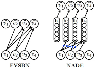
Figure: Architectural comparison between FVSBN (left) and NADE (right). FVSBN uses direct connections from all previous variables (v₁, v₂, v₃) to each output, resulting in O(n²) parameters. NADE introduces shared hidden layers (h₁, h₂, h₃, h₄) with weight tying - the blue arrows show how the same weight matrix W is reused across positions, dramatically reducing parameters to O(n) while maintaining expressiveness. (Source: Larochelle & Murray, 2011) ¹

Key insight: Instead of separate parameters for each conditional like FVSBN, NADE uses weight tying:

• Shared weight matrix $W \in \mathbb{R}^{d \times n}$ where $W_{\cdot,<i}$ takes first $i-1$ columns
• Each position has output weights $\alpha_i \in \mathbb{R}^d$ and bias $b_i$
• Total parameters: Linear in $n$ rather than quadratic

The architectural difference is clear from the figure: FVSBN has direct connections from all previous variables to each output, while NADE introduces a hidden layer that shares weights across positions, dramatically reducing parameters while improving generalization.

Concrete example: For MNIST with $d=500$ hidden units:

• FVSBN: $\sim 784^2/2 \approx 300K$ parameters
• NADE: $500 \times 784 + 784 \times 500 = 784K$ parameters but with better generalization

Connection to Autoencoders

At first glance, NADE looks similar to a standard autoencoder - both have an encoder that creates hidden representations and a decoder that reconstructs the input. However, there’s a crucial difference:

Standard Autoencoder:

• Encoder: $h = \sigma(W_2(\sigma(W_1 x + b_1)) + b_2)$
• Decoder: $\hat{x} = \sigma(V h + c)$
• Not generative: Cannot sample new data - it just reconstructs inputs

NADE (Autoregressive Autoencoder):

• Maintains autoregressive structure: $\hat{x}_i$ can only depend on $x_1, \ldots, x_{i-1}$
• Properly generative: Defines a valid probability distribution $p(x)$
• Sequential sampling: Can generate new samples by sampling $x_1$, then $x_2|x_1$, etc.

The key insight is that a vanilla autoencoder is not a generative model - it doesn’t define a distribution over $x$ that we can sample from to generate new data points. NADE solves this by enforcing the autoregressive property, making it properly generative while learning useful hidden representations as a byproduct of modeling the conditional distributions.

Masked Autoencoder for Distribution Estimation (MADE)

MADE ² solved a key computational inefficiency in NADE through a clever masking approach. While NADE can theoretically compute all conditional probabilities in parallel during training (since all input values $x_1, x_2, \ldots, x_n$ are known), the original implementation required separate forward passes for different conditioning sets.

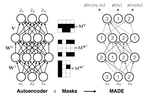
Figure: MADE uses masked connections to transform a standard autoencoder into an autoregressive model. The masks (shown in center) ensure that output $\hat{x}_i$ only depends on inputs $x_1, \ldots, x_{i-1}$, preserving the autoregressive property while enabling parallel computation. (Source: Germain et al., 2015) ²

MADE’s Key Innovation:

• Single forward pass: Computes all conditional probabilities $\hat{x}_1, \hat{x}_2, \ldots, \hat{x}_n$ simultaneously
• Masked connections: Binary masks ensure $\hat{x}_i$ only sees $x_{<i}$, maintaining autoregressive structure
• Standard architecture: Uses familiar autoencoder structure, making it easy to implement and scale

The Masking Mechanism:

1. Assign each hidden unit a number $m \in \{1, 2, \ldots, n-1\}$
2. Hidden unit $h_j$ with number $m_j$ can only connect to inputs $x_1, \ldots, x_{m_j}$
3. Output $\hat{x}_i$ can only connect to hidden units with $m_j < i$

This elegant solution made autoregressive modeling much more hardware-efficient and would later inspire the masked self-attention mechanism in Transformers.

Modern Transformers

Today’s language models like GPT follow exactly the same principle, just with more sophisticated architectures:

• Self-attention mechanisms for capturing long-range dependencies
• Massive parameter counts and training data
• Parallel training with causal masking
• But still fundamentally: $p(x_1,\ldots,x_n) = \prod_i p(x_i | x_{<i})$

Maximum Likelihood Learning and the KL Connection

How do we train these models? The standard approach is Maximum Likelihood Estimation (MLE), but there’s a beautiful connection to information theory that’s worth understanding deeply.

The Key Insight: Maximizing the likelihood of our data is equivalent to minimizing the Kullback-Leibler (KL) divergence between the true data distribution and our model’s distribution.

Let’s unpack that.

The Math: From KL Divergence to Maximum Likelihood

The KL divergence from our model’s distribution $P_\theta$ to the true data distribution $P_{\text{data}}$ is defined as:

$D_{KL}(P_{\text{data}} || P_\theta) = \mathbb{E}_{x \sim P_{\text{data}}} \left[ \log \frac{P_{\text{data}}(x)}{P_\theta(x)} \right]$

This formula measures the “divergence” of our model’s predictions from the true distribution. Let’s expand it:

The first term, the entropy of the data, is a fixed value. We can’t change it. Therefore, to minimize the KL divergence, we must maximize the second term: $\mathbb{E}_{x \sim P_{\text{data}}} [\log P_\theta(x)]$.

Since we don’t know the true $P_{\text{data}}$, we use our training dataset $D = \{x^{(1)}, \ldots, x^{(m)}\}$ as an empirical sample. This turns the expectation into an average:

$\arg \max_\theta \mathbb{E}_{x \sim P_{\text{data}}} [\log P_\theta(x)] \approx \arg \max_\theta \frac{1}{|D|} \sum_{x \in D} \log P_\theta(x)$

This is exactly the objective for Maximum Likelihood Estimation.

Therefore: Minimizing KL divergence is the same as maximizing the log-likelihood.

An Intuitive Guide to Information Theory

For those new to information theory, let’s build an intuition for these concepts using a simple example.

Imagine two people, Alice and Bob. Alice is flipping a coin and Bob is trying to guess the outcome.

• Entropy: This is the average amount of “surprise” or “information” in an event. If Alice’s coin is fair (50% heads, 50% tails), the outcome is maximally unpredictable. The entropy is high. If her coin is biased (e.g., 99% heads), there’s very little surprise, and the entropy is low. Entropy is a property of a single probability distribution. $H(p) = -\mathbb{E}_p[\log p(x)]$

• Cross-Entropy: Now, let’s say Alice’s coin is fair ($P_{\text{data}}$: 50/50), but Bob believes it’s heavily biased towards heads ($P_{\text{model}}$: 90/10). Cross-entropy measures the average surprise Bob experiences. He’ll be very surprised every time tails comes up, so the cross-entropy will be high. It measures the average number of bits needed to encode data from distribution $P$ when using a code optimized for distribution $Q$. $H(p,q) = -\mathbb{E}_p[\log q(x)]$

• KL Divergence: This is the extra surprise Bob experiences because his belief is wrong. It’s the gap between the cross-entropy and the true, minimal surprise (the entropy). It’s the penalty for using the wrong model. $D_{KL}(p||q) = H(p,q) - H(p)$

In our training scenario:

• $P_{\text{data}}$ is Alice’s true coin flip distribution (the real world).
• $P_\theta$ is Bob’s belief (our model).
• We want to adjust Bob’s belief (train our model $\theta$) to minimize his extra surprise (the KL divergence) when observing real-world outcomes.

The Asymmetry of KL Divergence: A Crucial Detail

A key property of KL divergence is that it’s asymmetric: $D_{KL}(P || Q) \neq D_{KL}(Q || P)$. This isn’t just a mathematical quirk; it has profound implications for how models are trained.

Let’s use our coin example again:

• $P$: True distribution (fair coin: 50% Heads, 50% Tails)
• $Q$: Model’s belief (biased coin: 90% Heads, 10% Tails)

Forward KL: $D_{KL}(P || Q)$ (What we use in MLE)

• We calculate the expectation over the true distribution $P$.
• We ask: “On average, how surprised is our model $Q$ when it observes data from the real world $P$?”
• The model is penalized for assigning low probability to events that are actually common. If $P(x)$ is high but $Q(x)$ is low, the term $\log(P(x)/Q(x))$ becomes very large.
• This is often called “mean-seeking” or “mode-covering”. The model tries to put its probability mass everywhere the true distribution has mass. It’s forced to predict both Heads and Tails to avoid infinite surprise.

Reverse KL: $D_{KL}(Q || P)$

• We calculate the expectation over the model’s distribution $Q$.
• We ask: “On average, how surprised would the real world be by our model’s samples?”
• The model is penalized for generating samples that are unlikely in the real world. If $Q(x)$ is high but $P(x)$ is low (or zero), the term $\log(Q(x)/P(x))$ becomes very large.
• This is often called “mode-seeking”. The model prefers to find one high-probability region in the true distribution and stick to it, even if it ignores other modes. It would confidently predict “Heads” and avoid the penalty of ever generating a “Tails” sample that is only 50% likely in reality.

Since we train generative models via Maximum Likelihood, we are implicitly using the forward KL divergence, $D_{KL}(P_{\text{data}} || P_{\text{model}})$. This encourages our models to be broad and cover all the variations present in the training data. (This holds true for the models we’ve discussed, which are trained via MLE. As we’ll touch on in the final section, other prominent generative models like VAEs and GANs use different training objectives that can lead to different behaviors.)

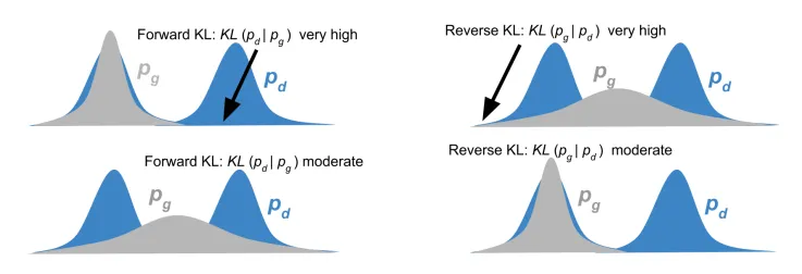
Figure: A visual comparison of Forward and Reverse KL Divergence. In Forward KL ($D_{KL}(P_d || P_g)$), the model $P_g$ (gray) must cover both modes of the true data distribution $P_d$ (blue) to avoid high penalties. In Reverse KL ($D_{KL}(P_g || P_d)$), the model can focus on a single mode of the data to avoid penalization for generating unlikely samples. (Source: Manisha & Gujar, 2018) ³

A Fundamental Limitation: Forward vs Reverse Factorizations

Here’s something that surprised me: different factorization orders can represent different hypothesis spaces.

Consider factoring a joint distribution $p(x_1, x_2)$ in two ways:

If we use neural networks with Gaussian outputs for each conditional, these can represent different sets of distributions!

Example: Suppose $p(x_1) = \mathcal{N}(0,1)$ and $p(x_2|x_1) = \mathcal{N}(\mu_2(x_1), \epsilon)$ where $\mu_2(x_1) = 0$ if $x_1 \leq 0$ and $\mu_2(x_1) = 1$ otherwise.

The marginal becomes:

$p(x_2) = \int_{-\infty}^{\infty} p(x_1) p(x_2|x_1) dx_1 = 0.5\mathcal{N}(0,\epsilon) + 0.5\mathcal{N}(1,\epsilon)$

This marginal $p(x_2)$ is a mixture of two Gaussians, which a single Gaussian $p(x_2)$ in the reverse factorization cannot represent. This shows that the hypothesis spaces are genuinely different.

From Theory to Practice: GPT-2 Implementation

Working with a GPT-2 model brings these concepts to life. The architecture follows our chain rule exactly:

1. Token Embeddings: Each of 50,257 possible tokens gets a 768-dimensional embedding
2. Transformer Layers: Self-attention and feed-forward networks process the sequence
3. Output Layer: Projects back to 50,257-dimensional logits for $p(x_i|x_{<i})$

Temperature Scaling

Temperature scaling provides an interesting way to control the sharpness of predictions:

$p_T(x_i|x_{<i}) \propto e^{\log p(x_i|x_{<i})/T}$

The temperature parameter $T$ has the following effects:

Interestingly, applying temperature scaling token-by-token doesn’t recover joint temperature scaling:

This is another manifestation of how different factorizations can lead to different behaviors.

The Bigger Picture: Why This All Matters

What strikes me most about this journey through autoregressive models is how a single mathematical principle - the chain rule - connects such a wide range of techniques:

1. Classical graphical models (Bayesian networks) use it with conditional independence assumptions
2. Early neural approaches (FVSBN, NADE) parameterize the conditionals with neural networks
3. Modern language models (GPT, etc.) scale up the same principle with massive architectures and data

The information-theoretic perspective provides the unifying learning framework: we’re always trying to minimize the “compression loss” when encoding real data using our model’s learned code.

Reflections and What’s Next

Understanding these fundamentals has been crucial for appreciating more advanced generative models. Variational autoencoders, GANs, and diffusion models all build on different approaches to the same core challenge: how to represent and learn complex, high-dimensional distributions.

It’s also crucial to recognize that the Maximum Likelihood approach, and its connection to forward KL divergence ($D_{KL}(P_{\text{data}} || P_{\text{model}})$), is characteristic of autoregressive models but not universal. Other major families of generative models are defined by their avoidance of direct likelihood maximization. For instance, Variational Autoencoders (VAEs) optimize a lower bound on the likelihood (the ELBO) which involves a reverse KL term, leading to different model behavior. Generative Adversarial Networks (GANs) bypass likelihood entirely, instead training via a minimax game whose objective relates to Jensen-Shannon divergence. These different training paradigms are a key reason why the “generative zoo” is so diverse and fascinating.

The autoregressive approach is particularly elegant because it’s:

• Theoretically grounded: Based on exact probability factorization
• Computationally tractable: Sequential generation and parallel training
• Empirically successful: Powers today’s best language models

For anyone diving into generative modeling, I’d recommend really understanding this foundation before moving to more complex approaches. The chain rule isn’t just a mathematical identity - it’s the key that unlocks scalable generative modeling.

This post represents my understanding from working through the foundational concepts of generative modeling. If you spot any errors or have questions, I’d love to hear from you!

References